Hyperspectral Inverse Skinning

Presentation

Eurographics 2021: [YouTube], [Keynote (70 MB)], [PDF (20 MB)], [PDF with notes (20 MB)]:

Abstract

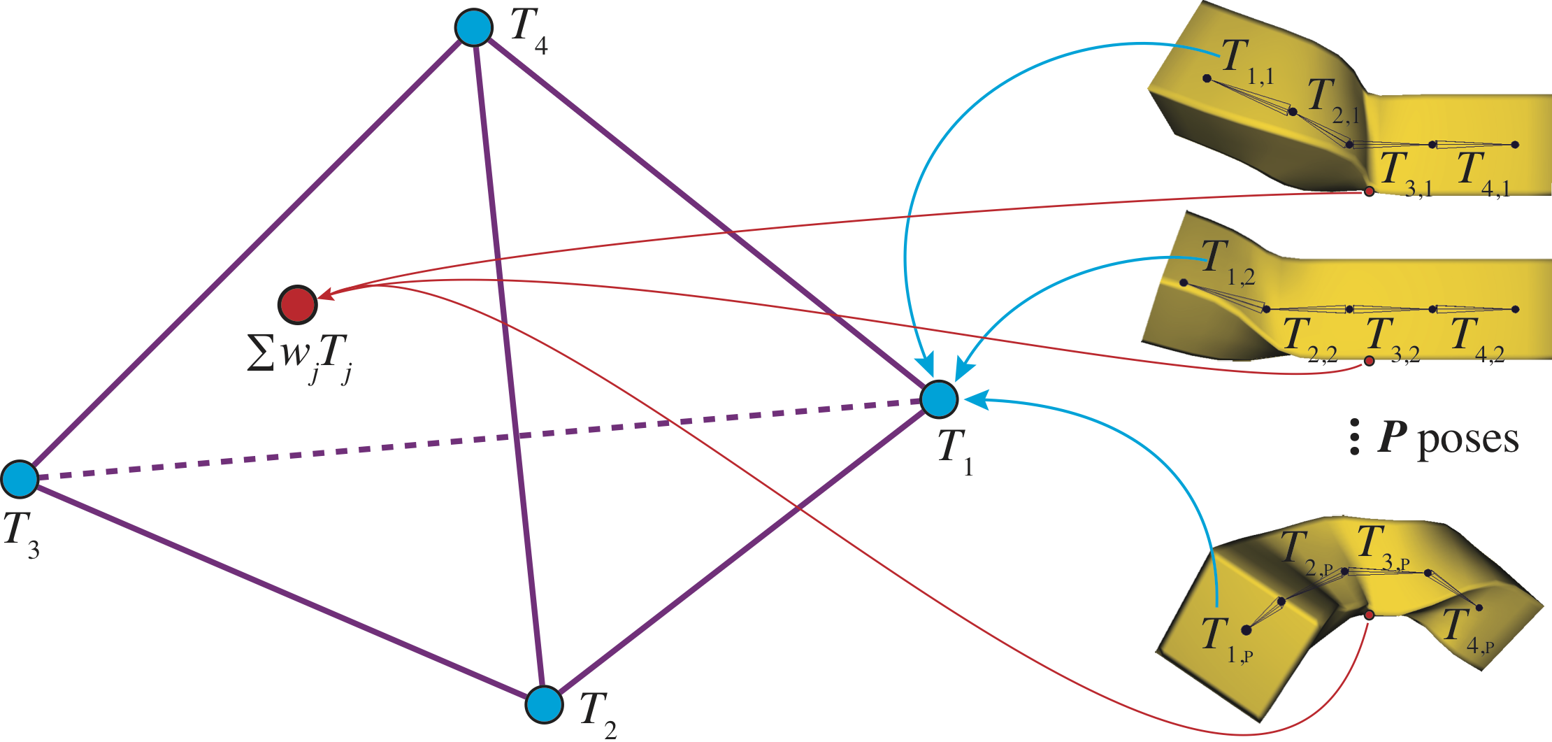
In example-based inverse linear blend skinning (LBS), a collection of poses (e.g., animation frames) are given, and the goal is finding skinning weights and transformation matrices that closely reproduce the input. These poses may come from physical simulation, direct mesh editing, motion capture, or another deformation rig. We provide a re-formulation of inverse skinning as a problem in high-dimensional Euclidean space. The transformation matrices applied to a vertex across all poses can be thought of as a point in high dimensions. We cast the inverse LBS problem as one of finding a tight-fitting simplex around these points (a well-studied problem in hyperspectral imaging). Although we do not observe transformation matrices directly, the 3D position of a vertex across all of its poses defines an affine subspace, or flat. We solve a “closest flat” optimization problem to find points on these flats, and then compute a minimum-volume enclosing simplex whose vertices are the transformation matrices and whose barycentric coordinates are the skinning weights. We are able to create LBS rigs with state-of-the-art reconstruction error, and state-of-the-art compression ratios for mesh animation sequences. Our solution does not consider weight sparsity or the rigidity of recovered transformations. We include observations and insights into the closest flat problem. Its ideal solution, and optimal LBS reconstruction error, remain an open problem.

Paper

Code and input (ground truth) data

Data

Much of the data can be found in the GitHub repository. Some data in convenient formats are snapshotted here.

• Ground truth input meshes animations (mostly from previous work) [442 MB zip]
• Ground truth linear blend skinning rigs for our new ground truth examples [26 MB zip]
• Output OBJs recovered by our approach [355 MB zip]
• Subset of output OBJs recovered by Le and Deng [2012] [65 MB zip]. (All output is in the GitHub repository in their TXT format.)
• Output OBJs recovered by Luo et al. [2019] [602 MB zip]

Comparison Videos

These videos show our algorithm's reconstructed output next to the input and Le and Deng [2012]'s SSDR technique (without rigidity constraints). We render with flat shading to accurately portray surface quality.

• samba.mp4
• horse-collapse.mp4
• elephant-gallop.mp4
• crane.mp4

Optimization Visualizations

Cylinder optimization visualizing closest points in the 3D handle subspace

These videos all visualize our bi-quadratic flat optimization on the cylinder example, which has a known ground truth solution. (See Figure 10 in the paper.) There are four bones, each the vertex of a tetrahedron, so the desired handle flat is 3D. Each point is shown in the visualization is the closest point on the handle flat to each vertex's flat. Because the orientation of the visualized 3D space is arbitrary, (obtained via PCA from the ambient 48-dimensional space), we apply a procrustes transformation between adjacent iterations.

Two videos show optimization from a random initial guess. This optimization never achieves the known ground truth and never stops changing, even after 10451 iterations. One video shows all 10451 iterations at 50x real-time. The other video shows the beginning iterations at a slower speed (4x real-time).

• biquadratic optimization from random initial guess (10451 iterations at 50x speed).m4v
• biquadratic optimization from random initial guess (beginning iterations at 4x speed).m4v

One video shows our optimization from our proposed initial guess (the 50th percentile case in Section 4.1, Table 2). It quickly converges to the ground truth within 20 iterations.

• biquadratic optimization from proposed initial guess (Section 4.1, Table 2, 50th percentile).mov

Another video shows our optimization from an alternate initial guess (the 10th percentile case in Section 4.1, Table 2). It eventually reaches the ground truth after ~300 iterations.

• biquadratic optimization from alternate initial guess (Section 4.1, Table 2, 10th percentile, 310 iterations at 4x speed).m4v

Line-line optimization in 3D

A video of flat-flat optimization iterations for the scenario in 3D in which the given and unknown flats are lines (1D). There is a known zero-energy solution. The optimization algorithm is the explicit p,B parameterization, optimized using the Hessian-based trust region solver constraining B to lie on the Grassmann manifold. The optimization quickly reaches the known solution.

• line-line optimization in 3D (p,B manifold optimization).mp4

BibTeX

@article{Liu:2020:HIS,
 author    = {Liu, Songrun and Tan, Jianchao and Deng, Zhigang and Gingold, Yotam},
 title     = {Hyperspectral Inverse Skinning},
 journal   = {Computer Graphics Forum (CGF)},
 volume    = {39},
 number    = {6},
 pages     = {49--65},
 year      = {2020},
 doi       = {10.1111/cgf.13903},
 keywords  = {linear blend skinning, deformation, animation, affine geometry, hyperspectral unmixing}
}

Funding

This work was supported in part by the United States National Science Foundation (IIS-1453018 and IIS-1524782), a Google research award, and a gift from Adobe Systems Inc.